Deciphering Quanta

Sometimes it is claimed that Quanta articles are so watered down of mathematical content that they become meaningless. That presents a challenge: do I understand the quanta article on my own work?

Here goes:

New Proof Distinguishes Mysterious and Powerful ‘Modular Forms’

I can confirm that I did not see this article in any form before it appeared. Overall I would say that it is faithful to the facts and I can interpret what everything means. I’m not quite sure why there is an Alex Kontorovich explainer about the Langlands Program in there but why not?

I did, however, have to stop and wonder when I saw the following picture:

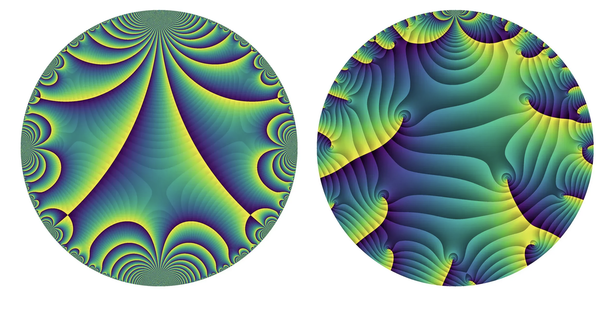
This appeared with the caption *Congruence modular forms (left) have additional structure that noncongruence modular forms (right) lack.* OK, here is the challenge: can I work out what this picture actually represents?

In both pictures, there is clearly some color gradient between yellow and blue, and this has discontinuities along some regions we call \(L\) and \(R\) for left and right. These are also clearly pictures inside \(\mathbf{H}^2\) in the Poincaré disc model.

Here \(L\) looks at least superficially like a fundamental domain for some Fuchsian group. The rays of \(L\) going towards the point \(i\) on the boundary do look like geodesics in the hyperbolic metric (which are circular arcs meeting the boundary at right angles). There is a corresponding invariance for the figure by the parabolic element (with some cusp width) through \(i\). Consider a conformal map from the upper half plane to this model which sends \(\infty\) to \(i\):

Using the standard conformal map with the upper half plane:

\(\phi: \mathbf{H} \rightarrow D(0,1), \quad z \mapsto \displaystyle{\frac{1 + i z}{1 + z}} \)

From the picture, we see the images of the geodesics from the infinite cusp to \(n \alpha\) for \(n\) odd. All parabolic elements are conjugate, but if we are to guess what \(\Gamma\) is by looking at the picture then working out \(\alpha\) for this specific model is important. I tried to eyeball it for a while before printing it out and trying to compute the angle using continued fractions, which wasn’t so accurate but gave \(\tan \theta \sim 1/(1 + 1/3)\) with \(\theta\) in the mid \(30\)s. Then using some angle tools in keynote it came out to somewhere between \(36\) and \(37\) degrees, closer to the latter. So maybe it was exactly a \(10\)th root of unity, which would make \(\alpha\) live in a degree \(4\) field, or (much better!) maybe \(\alpha = 1/2\) in which case the angle is \(36.8698 \ldots\), and then \(L\) (or rather \(\phi(L)\) is invariant under exactly

\(A = \left( \begin{matrix} 1 & 1 \\ 0 & 1 \end{matrix} \right).\)

Maybe I should have guessed this in retrospect! Let’s look at the geodesic from \(i \infty\) to \(1/2\), which in the picture goes from \(i\) to \(4/5 – 3i/5\). There appears to be a point with \(4\)-fold symmetry. That suggests invariance under some order four element corresponding to an elliptic point. But this is a little worrying, since \(\mathrm{PSL}_2(\mathbf{Z})\) does not have any elements of order \(4\)! Now there are some ways around this. For example, this could be the level set of a function which satisfies an extra invariance property under the normalizer of some congruence subgroup, and so does not itself come from an element of \(\mathrm{SL}_2(\mathbf{Z})\) but \(\mathrm{GL}_2(\mathbf{Q})^{+}\). For example, the Fricke involution on \(X_0(N)\) is \(\tau \mapsto -1/N \tau\) which corresponds to. a matrix in \(\mathrm{GL}_2({\mathbf{Q}})\) with determinant \(N\), although that has order \(2\). Any element of order \(4\) has to have eigenvalues of the form \(\alpha\) and \(\alpha i\), with \(\alpha + i \alpha \in {\mathbf{Z}}\), and thus eigenvalues \(1+i\) and \(1-i\) up to rational multiples. That means the determinant should be \(2\) times a square. The unique element such element up to conjugacy is

\(S = \left( \begin{matrix} 1 & 1 \\ 1 & -1 \end{matrix} \right)\)

which has order \(4\) and fixes \(i\). If we want to fix a point on the geodesic \(1/2 + i t\), we can just make a hyperbolic scaling and then conjugate to get the matrix

\(S_t = \left( \displaystyle{ \begin{matrix}
1 – 1/2t & t + 1/4t \\
-1/t & 1 + 1/2t \end{matrix} } \right).\)

Here I started to run into a problem because it’s hard to approximate \(t\) to any precision from the picture, although \(t \sim 0.1\) numerically. There are a few natural integral matrices one can write down but it wasn’t clear what was going on.

Next I turned to the picture around the cusp \(-i\). This looks kind of weird because the biggest curves decidedly do not look like geodesics. But if we ignore this, we might decide that \(-i\) is another cusp. It’s also disturbing that the fundamental domain appears to contain enough of the boundary to suggest that \(\Gamma\) is a thin group, but let’s ignore this as well. So what is the cusp width (with out normalizations) at \(-i\)? Here numerically I simply get nonsense.because if there really were geodesics around \(i\) translated by a fixed parabolic element and the first one was of the size indicated in the picture then there would be many fewer visible ones. As a typical example, one should expect a picture like this:

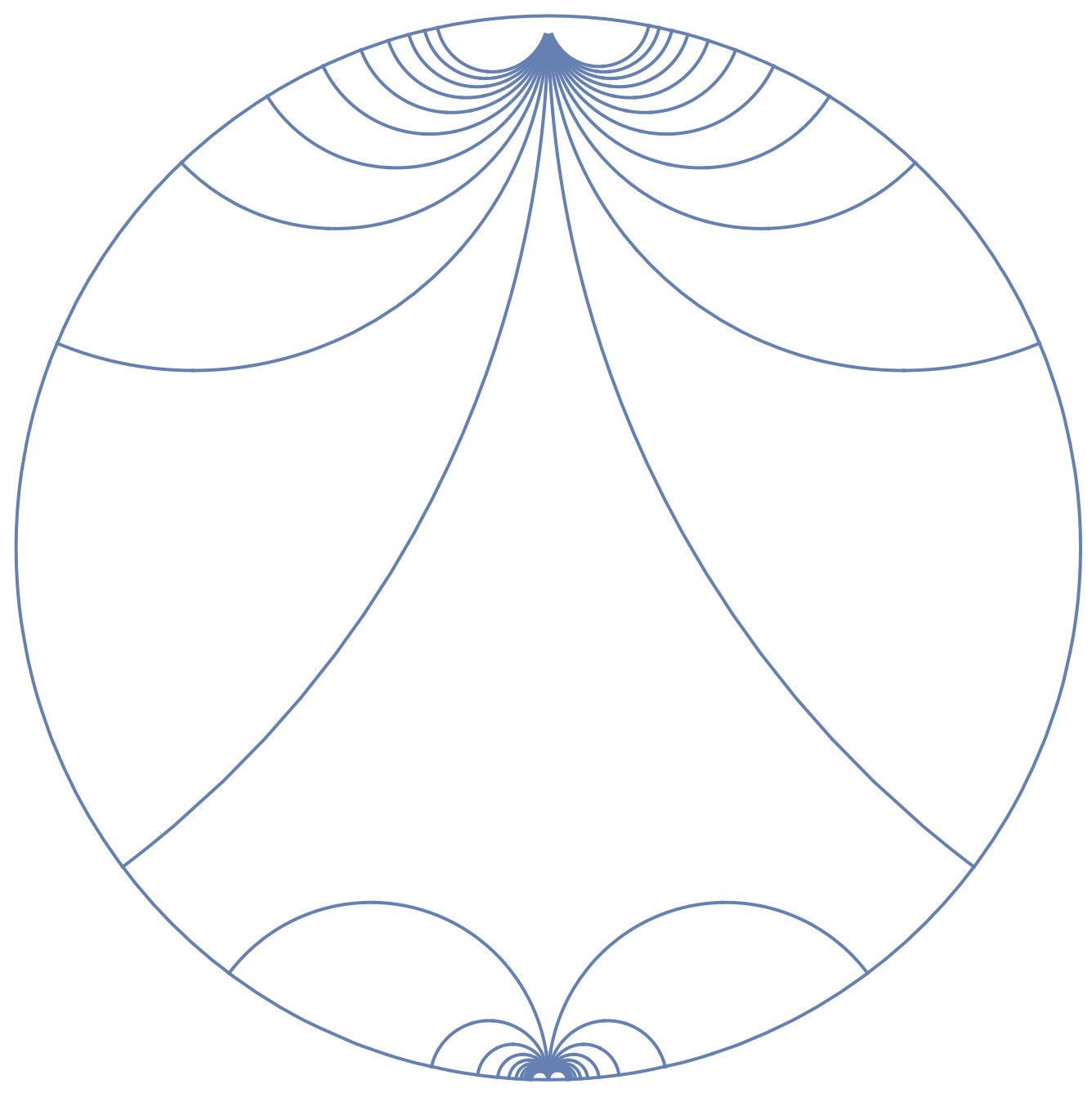
which doesn’t look anything like the original picture.

So I’m ready to give up now. What about the picture on the right? Well here I don’t even know how to begin. There is not any obvious evidence of parabolic elements, which are not only present in congruence subgroups of \(\mathrm{SL}_2(\mathbf{Z})\) but of any non-congruence subgroup as well. Perhaps there is a cusp at \(i\) with some large cusp width. There also seem to be singularities inside the disc. But that just suggests this might be a level set of a meromorphic form. But why choose a meromorphic form rather than one that is holomorphic away from the cusps? I wonder if that gives hints about the first picture; perhaps the transition from yellow to blue occurs when \(\mathrm{Im}(f)\) goes from positive to negative, and where it might be \(0\) along some geodesic arc (For example: the Fourier coefficients are rational so the form is real along the purely imaginary axis) but the form can also have imaginary part \(0\) along some non-geodesic regions and that is what one is seeing around \(-i\). That might allow one to reinterpret the graphs as something related to \(\mathrm{Im}(f)\). This suggests that the point on the left that appears to have degree four instead is related to a “local” symmetry coming from a vanishing point of the derivative of the modular function, but I’m just guessing now.

I should probably spend no more time on this, so instead I open up speculations to the comments!

Full Disclosure The picture comes with an attribution to David Lowry-Duda but I did not try to follow that lead.

Update: Perhaps it was not as obvious as intended, but the request for speculation was intended to be “how do you interpret this from the picture alone” not “send me a link” which is something which I deliberately avoided trying to do. (I will no doubt look at the way they are generated at some point in more detail.) A brief look at the LMFDB link suggests that my second explanation is pretty close, although the graph on the left is of the argument of a modular function (or rather the modular form \(\Delta\)) rather than the imaginary part. But the guess as to the explanation for the “order four” symmetry is correct, it is explained by the vanishing of \(\Delta'(\tau)\) or equivalently the vanishing of \(E_2(\tau)\) at a point on the geodesic \(1/2 + i t\). The picture on the right is still a mystery, however, and original speculations are still welcome.

Update II: So here is an new example. Like the graphs above, it plots the argument of a two modular forms on (different) finite index subgroups of \(\mathbf{SL}_2(\mathbf{Z})\). I have normalized both pictures so that the cusp width at the cusp \(i\) is the same in both cases (under the normalizations above invariant under \(\tau \rightarrow \tau + 3\); making the cusp width too small makes the behavior at \(tau = i \infty\) dominate the picture as the covolume goes up. There are dome differences with this example however:

1. I have used (holomorphic) modular functions rather than modular forms.
2. For these particular choices of functions, they are non-zero everywhere.
3. I made the picture myself so it is not as pretty as the ones above.
4. The functions I chose have the property that they are real precisely on geodesics, and thus the singularities here do form a tesselation.

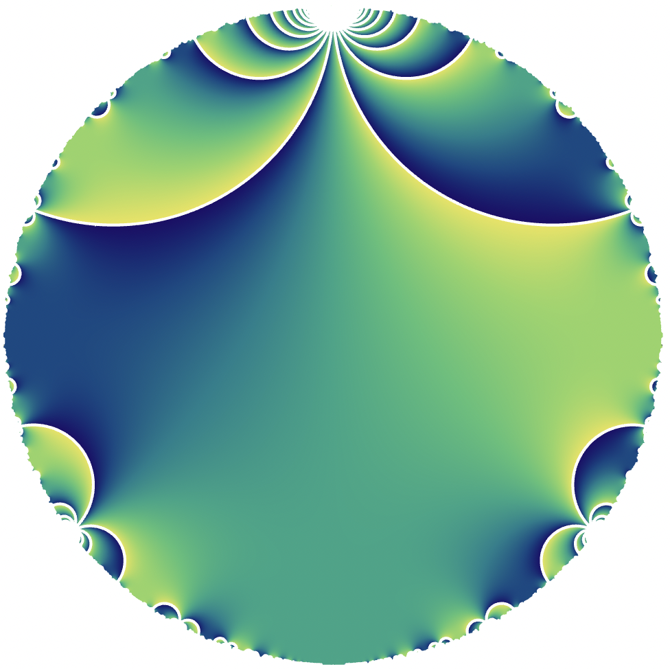
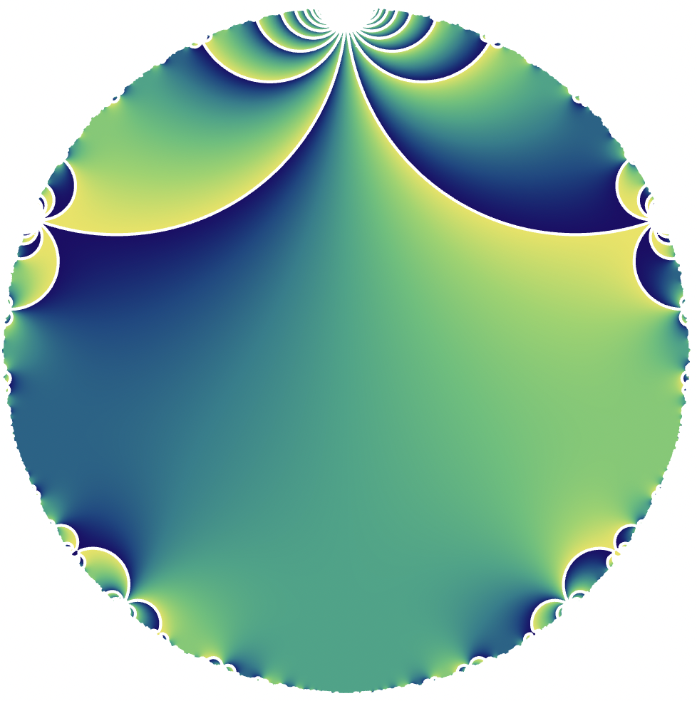
Now one of the forms is defined on a congruence subgroup and has a Fourier series in \(\mathbf{Z}[[q]]\), the other has a Fourier series in \(\mathbf{Q}[[q]]\) but not in \(\mathbf{Q} \otimes \mathbf{Z}[[q]]\) and is only defined on a non-congruence subgroup. But which is which? The pictures here are clearly much more similar than the pair of pictures above!